Introduction
During the 1980s, a few researchers and collaborators including Yann LeCun, one of the prominent figures in the field of AI, proposed a neural network architecture inspired by the Neocognitron model, a specific neural network architecture inspired by biological visual systems. The team developed a computational model and proposed the algorithm for training it to recognize handwritten zip codes. This neural network model, devised by Yann LeCun and his team, not only displayed exceptional accuracy in recognizing handwritten digits but also efficient training times. Later, this model got widespread adoption and many of them began using it for Benchmark Image Recognition tasks.
Fast forward to today, and the adoption of this remarkable neural network architecture, known as Convolutional Neural Network (CNN), has led to greater achievements in object detection, surprisingly reaching an accuracy level of 95%. This number is quite strange since 95% accuracy means surpassing the human ability for recognizing objects!. This incredible capability of CNN makes it ideal for all sorts of Computer Vision tasks including Face recognition, Object Detection, Medical Imaging, etc, and even help to generate images. So if you are starting out with Computer Vision, knowing how CNNs work will be a good foundation for your journey. To learn how this Neural Network works in detail, follow this entire article and the upcoming articles which discusses everything in deep about CNNs. However, This article will delve into the basics of Convolutional Neural Networks (CNNs) and explore step-by-step their architecture, working principles, and applications. Let's get in.
1. CNN: The Biological Perspective
We said CNNs are great for computer vision tasks, but how? Well, this question can be approached from two perspectives: the mathematical perspective and the biological perspective. Let's discuss the biological perspective. CNNs are inspired by the working of the mammalian visual cortex specifically the primary visual cortex or V1. V1 is the region in the brain that is responsible for processing visual inputs at a higher level. Scientists have discovered that neurons in the primary visual cortex (V1) respond to specific patterns of light rather than processing the entire image as a whole. V1 also has a lot of simple and complex cells for processing visual input. The simple cells are used for extracting the basic features of the visual input and then the complex cells find complex features and patterns. For example, consider the image of a chair, When you are seeing a chair, your V1 is not processing the entire image of the chair, instead, it finds the features that make it a chair, including the four legs and the backrest which can be detected by your simple cells. But what if you are seeing a sofa? Well, the sofa also has four legs and a backrest, but you have no trouble recognizing it as a sofa. This is done by your complex processing mechanisms in the primary visual cortex. It finds that an object with four legs, a backrest, and a wider shape can be a sofa while a shorter width can be a chair. The same idea goes to CNN. Instead of processing the entire image which is relatively complex, CNN finds specific features one by one and finally detects the image.
2. How CNN Can Be Ideal for Computer Vision?
CNNs have lots of advantages when comes to Computer Vision tasks, The main advantage is the one we have discussed above known as Hierarchical Learning. Hierarchical Learning allows CNN to extract low-level features from the image and gradually learn more complex patterns and features as it propagates through multiple layers similar to the way V1 works. Some other features include,
2.1 Parameter Sharing:
The core of CNN is the weights also known as parameters, But what makes CNNs special from traditional neural network layers is that the weights are shared in the first few layers. When considering the case of an image, the CNN works on local receptive fields, which means, each neuron in the first few layers of CNN is connected to a small region of the input image, and the network learns the parameters in this particular region. The same set of weights is used across all the neurons in the particular receptive field. This improves CNNs generalization capabilities and can detect specific features in the image.
2.2 Sparse Connectivity:
In traditional Neural Network architecture, each of the neurons has a connection to each of the previous neurons, or we can say, each of the output neurons is connected to each of the input neurons. But this is different in CNNs. In CNN, there is sparse connectivity or sparse interactions. In this technique, the weight matrix is typically much smaller than the input matrix. This enables us to find some specific regions of the image which are really important and avoid the rest which are insignificant. For example, if you want to detect a cat's picture from a group of animals from a single frame, you don't really need to consider all the other animals, only the cat's features
2.3 Downsampling:
CNNs have a particular layer known as Pooling. Pooling Layers helps to reduce the number of dimensions (downsampling) while preserving important features. This helps to reduce the computational complexity and increase the efficiency of the network on large datasets.
These are some of the features of Convolutional Neural Networks that make it ideal for Computer Vision tasks.
3. The Architecture of Convolutional Neural Networks
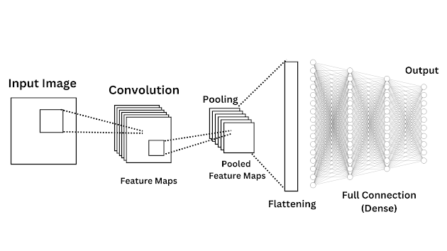
The architecture of Convolutional Neural Networks consists of several layers, Including Convolution, Activation (ReLU) Layer, Pooling, Flattening layer, and Fully connected layer. Don't worry we'll discuss each of these layers in detail. Here is the simple diagrammatic representation of each of these layers.
| CNN Architecture, Fig: 1 |
3.1 Convolution Layer: The heart of CNN
Let's discuss the primary and the most important layer in CNN, The Convolution Layer. The basic operation in the Convolutional Layer is of course Convolution, an important mathematical operation that has several applications. It is one of the important operations in signal processing and has also proven to be effective in Image data. Here is the formula of Convolution:
Convolution in mathematics is an operation that combines two functions to produce a third function that represents how one function modifies the other. This makes sense when comes to image processing since we are convolving the image data to produce a new output that represents the nature of the two functions. The convolution operation is typically represented by an asterisk (*) symbol. This representation above is basically in terms of CNNs terminology, Here, the is known as the input, and is known as weights, or we can call it filters or kernels. These filters or kernels are those that we are using to convolve with the image data. The parameter represents the spatial location within the input image.
However, this is not how we exactly represent the Convolution operation in terms of CNN, There are two things to note, first some of the fancy terms here are not directly used in CNNs, I showed this to get you an idea of the Convolution operation. Second, this equation is used for continuous inputs, In the case of signal processing we actually deal with continuous inputs, but in Image processing, there is only a discrete number of pixels, so the simply changes to the , meaning that the combined integration of two function changes to the summation of the corresponding elements.
Still, this is a fancy notation, let's break it down to the actual equation of Convolution in CNN,
Does this equation seem more terrifying? Not at all, The is our input or we can say a 2-dimensional image and the is the Kernel which is also 2D. What about the indices? The are indices that are used to represent a single pixel in the input image, kernel, and the produced output. are used to represent the dimensions (height, width) of the filter or kernel. The, represents the specific pixel value of the input image at the position . As and change, the filter is applied through each of the input pixels. Now, there are two sums, and the outer summation is used to slide the kernel over the input image which iterates over from 0 to slides vertically over the input image. Meanwhile, the inner summation is used for element-wise multiplication which iterates over from 0 to , representing the horizontal sliding of the kernel over the image. Finally, a bias term is added for providing flexibility for the network.
Here is an animation of convolution done on an image matrix of shape 3x4 with a kernel 2x2,
| Convolution, Fig: 2 |
This seems simple and straightforward, In an image of 3x4 pixels and a Kernel that we choose to be 2x2 as shown in the animation, the kernel is applied to each of the specific 2x2 spots of the input image. Each individual pixel is multiplied by the corresponding kernel value in each spot and the results are added together to produce the output pixel. This selected spot is known as the respective field of the image and sliding through each of these respective fields one by one is known as a stride. The stride value can be adjusted according to the desired movement, such as 1, 2, 3, or any suitable number. In our case, a stride of 1 is used, as seen in the animation where the respective field slides one pixel at a time. However, the stride can be modified for different patterns or requirements.
You can also connect the animation with the equation of the convolution we have discussed. The kernel is sliding over the input image one stride at a time. On each sliding, the element-wise multiplication is performed finally producing the output at the right side. This whole thing is the Forward Pass in the Convolution Layer of CNN.
Remember we have told about Sparse Connectivity and Parameter Sharing, We can find these two when looking at the animation, Here only the selected number of weights or kernels are applied to the image during the convolution process. Instead of connecting every single weight to all the pixels in the input image, This is an example of Sparse Connectivity and Parameter Sharing.
Sometimes, the output produced from convolving the image is referred to as Feature Map. There can be multiple numbers of feature maps which depends on the number of kernels used. If there are multiple kernels used, then there must be the same number of feature maps produced after convolution. Typically, we use multiple kernels in CNN for detecting multiple patterns or features in the input image. Each kernel focuses on detecting a specific pattern or feature, such as edges, textures, or shapes. When these kernels are convolved with the input image, they generate corresponding feature maps, with each feature map capturing the presence and location of a particular pattern or feature.
What Really Happens in Convolution?
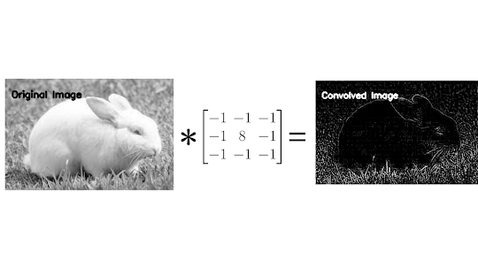
So we have discussed the intuition behind the Convolution Layer which includes the output(feature maps) produced on Convolving input image and kernels. But what exactly is Convolution doing in the actual sense? Let's consider a grayscale image of a cute bunny and try to figure out what convolution really does,
| Convolved Image (Grayscale), Fig 3 |
Which one makes more sense to you? Might be the one on the left, this is because your brain itself has created a mental model over time, allowing you to perceive and interpret visual information with ease. However, in the realm of computers, this ability doesn't come naturally. Computers need instructions and algorithms to create a model which can interpret visual data. Here, Convolution will help us. As you can see in the convolved image, the edges of the bunny are clearly visible, also the bunny's small eye, wide ears, etc. These are some of the features that make a bunny a bunny, So convolution can help to extract meaningful features from an image that can be learned.
Now, one more thing to understand, the output or feature map produced after convolving an image depends upon the kernel used, For different kernels, you'll get different results. This is not something we need to care about since kernels are learned by CNN itself during the training process, and that's the beauty of CNN, It finds the features it sees as more important which sometimes makes no sense to humans.
| Convolved Image with the kernel, Fig: 3 |
3.2 Activation Layer
CNN has several stages, the first stage as we discussed is the convolution operation, here multiple feature maps are produced by performing several convolutions. In the second stage of CNN, we need to transform the linear feature maps obtained from the convolution operation into a non-linear representation. This is achieved through the application of an activation function. In most cases, we use ReLU (Rectifier Linear Unit) as the activation function in the activation layer thus this layer is sometimes known as ReLU Layer. If you want to know more about the popular activations functions used in Neural Networks, check out this article
ReLU is a simple activation function that returns zero if the value is zero or less than zero else returns the original value. Now you can guess what ReLU does when we pass the entire output of convolutions.
| ReLU Applied to Convolved Image, Fig: 4 |
The changes in the image after applying the activation function (such as ReLU) depend on the specific features present in the input image and the weights of the convolutional kernels.
In some cases, the activation function may introduce non-linearities and enhance certain features, resulting in noticeable changes in the image. For example, if there are areas of low intensity in the input image, applying ReLU activation can effectively remove them by setting their values to zero. This can lead to a more pronounced contrast and clearer edge detection in the resulting image.
However, it's also possible that the activation function may not introduce significant changes if the features in the input image are already well represented by the convolved features. In such cases, the activation function may simply maintain or slightly modify the existing features without dramatic alterations.
3.3 Pooling Layer
Now, Pooling is another important step in CNN, In this stage a pooling function is applied to the output of convolutions to modify it further. But why do we need to apply pooling? Well, there are lots of benefits to applying pooling in our CNN although it is not necessary. So let's discuss when and why to apply pooling.
Let's say you got some colorful HD images of cats and dogs and you need your CNN to classify them correctly. In the first stage, convolution is applied to the images producing feature maps, but sometimes there may be too many features extracted from the image which makes CNN utterly confused and can lead to overfitting. Here quality is better than quantity again, both a very small number of features and too many features are bad for CNN. So in our case, since the image is HD and colorful, there might be too many features extracted from the convolution operation that we need to select the most relevant information for classifying the images, here pooling will help us.
Pooling will help CNN to extract more relevant and quality features from the image containing too many features and significantly reduce the amount of computational power required to process the images, then these extracted features from pooling can be passed forward to a full connection layer to classify the images.
Now, there are different types of pooling,
3.3.1 Max Pooling:
In max pooling, a window slides over the input feature map produced after convolution, and the maximum value within each window is selected as the output. It helps in capturing the most dominant features and reducing the spatial resolution of the feature map. Let's consider the output produced after convolving the image like this (see Fig: 2)
When applying max-pooling of shape 2x2 and stride 1, we'll get,
3.3.2 Average Pooling:
In average pooling, similar to max pooling, a window slides over the input feature map. However, instead of selecting the maximum value, it computes the average of the values within each window. Average pooling helps in capturing a more general representation of the features.
When considering the same feature map, if we apply average pooling with shape 2x2 and stride 1, we'll get,
When considering the same feature map, if we apply average pooling with shape 2x2 and stride 1, we'll get,
3.3.3 Global Pooling:
Global pooling, which can also be global average pooling or global max pooling, aggregates the entire feature map into a single value. It computes either the average or maximum value across the entire spatial dimensions of the feature map. Global Pooling will reduce the dimensions significantly which also reduces the number of features in the feature maps, So it is not well-suited for sensitive feature images, But can be applied for summarizing the entire feature map.
In the case of Global Max Pooling, the largest value from the entire matrix is selected, In our case the result of Global Max Pooling is .
When comes to Global Average Pooling, the average of all the elements in the feature map is calculated, In our case the result of Global Average Pooling is
3.3.4 Min Pooling:
As the opposite of Max Pooling, a window slides over the input feature map produced, and the minimum value within each window is selected as the output. It can be used in cases where we need to find the least prominent features in the image.
3.3.5 Sum Pooling:
Sum Pooling simply calculates the sum of the pooling region. A window slides over the input feature map and then the sum of all the values in that region is calculated. Sum Pooling can be usually applied when we want to consider more features rather than selecting only the most important features.
These are some of the Popular Pooling techniques that can be used in CNN after applying the Convolution, Well, these are just examples, the real scenario can be different.
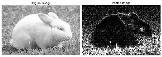
Let's see what happens if we apply Max Pooling to the Bunny image,
| Pooled Image, Fig: 5 |
3.4 Flattening Layer
Until now from Convolution, Activation, and Pooling we have worked with 2-dimensional matrices, In the Flattening Layer this entire 2D matrix is converted to a single 1D array known as Flattening. Flattening is used to feed the produced outputs to a fully connected Neural Network such as a Feed Forward Neural Network, this allows the entire CNN to learn the features and classify them accordingly.
Flattening Layer is one of the simplest steps in CNN. To illustrate, let's consider an example where we have passed some input through each layer of the CNN and got a result like this,
When this matrix is flattened it will look like this,
3.5 Fully Connected Layer (Dense Layer)
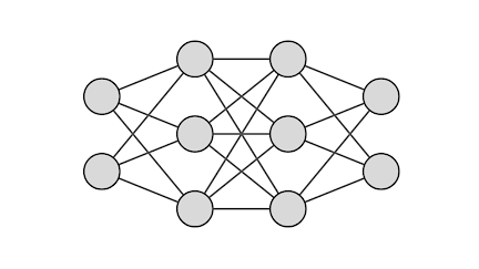
The Fully Connected Layer, also known as the Dense Layer, shares similarities with the Multi-Layer Perceptron (MLP) and can be considered an example of an MLP. In the Fully Connected Layer, each neuron is connected to every neuron in the previous layer, forming a fully interconnected network. The term "Fully Connected" is specifically used in CNNs to distinguish it from other layers we have discussed. Unlike convolutional and pooling layers that share weights across inputs, the Fully Connected Layer assigns unique weights to each input value.
| Fully Connected Neural Network, Fig: 6 |
The Fully Connected Layer serves as the Decision-making or classification layer in the Convolutional Neural Network. In this layer, the features detected by the preceding layers are passed for classification. The output of each neuron in this layer is computed as the weighted sum of inputs, which can be expressed as follows:
Where, W = Weights and X = inputs from the preceding layer, Φ = Activation function.
Maybe you felt like the equation for Convolution and Full Connection looks similar, that's right. But the difference is that Convolution operates on 2D matrices, where a kernel is applied to an input matrix through element-wise multiplications and summations while the fully connected layer works with 1D matrices or vectors.
Architecture In terms of RGB Images: Capturing Rich Visual Inputs
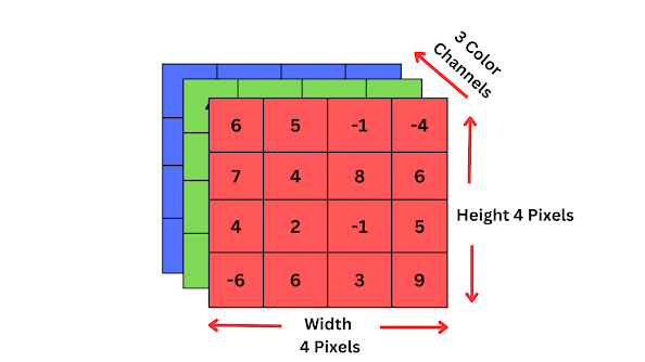
So far, everything we have covered is the fundamentals of how each layer operates in grayscale images, Now let's also discuss in terms of RGB. Things can be quite different when comes to RGB(Red, Green, Blue) colored images. Since RGB images have three color channels (red, green, and blue), we need to consider 3 input channels while grayscale images have a single channel representing the grayscale intensity.
| RGB Channels, Fig: 7 |
The operations performed in each layer of a convolutional neural network (CNN) remain the same for RGB (Red, Green, Blue) colored images, with the key difference being that these operations are applied to each of the three input channels separately. Rather than working with a single grayscale channel, we process RGB images by considering the information present in each color channel individually. This means that convolution, activation functions, pooling, and other operations are still performed, but they are applied independently to the red, green, and blue channels.
Usually, when RGB is involved we use a 3D Tensor to represent the height, width, and the color channels. Now if you are not familiar with tensors, that's ok we are not going deep into tensors now, but will surely discuss it in the upcoming articles since it is important. Now let's see an animation of how the Convolution is applied to RGB images to produce feature maps,
| Convolution in RGB, Fig: 8 |
It is not always mandatory, to sum up the outputs of RGB channels to generate a single output. While combining the outputs by addition can provide a more comprehensive representation from multiple channels, it is not always necessary. The decision to combine or treat the channels individually depends on the specific tasks. Analyzing each channel separately allows for individual feature extraction. Therefore, the choice depends on the desired outcome and the nature of the use case.
Now after producing the output, the rest of the operations are the same, Pooling, Flattening, Full Connection, etc.
Summing Up
| Summary Animation CNN, Fig: 9 |
So, that's it! we have done a very in-depth introduction and overview of Convolutional Neural Networks (CNN), All of the things we have discussed is just half part of CNN, this entire article is about the forward pass of inputs through Convolutional Neural Network, However, learning in CNNs involves updating the weights using Gradient Descent, a process known as backpropagation. In our next article, we will delve into the intricacies of backpropagation in CNNs, discussing the mathematics and logic behind it.
Thanks for reading!
Books:
Research Paper:


.gif)

